Adjustment with observation equationsAccuracy of adjusted, unmeasured height differences
For a connected vertical network specify the list of points with known heights. The input of the two to four columns complies with the general rules of tabular input. The pointnames may be chosen as in the . Coordinate lists may be transfered from other computation tools.
If heights should be subject to adjustment, please specify an accuracy measure, either a standard deviation or a weight. If a default value is given for the accuracy measure, it pads all missing values in this column. Otherwise all heights without accuracy measure are treated as error-free in the adjustment. This is equivalent to zero standard deviation. A list may consist of both adjustable points and fixed points.
Points not present in the network are ignored. Points without height and network points missing in the list are treated as new points. A free vertical network consists exclusively of new points, e.g., if the list of known points is empty.
If you specify coordinates X and Y then the vertical network is displayed on the canvas. Points without X and Y are not displayed. These coordinates are not used for network adjustment. If new points should be displayed on the canvas, then you must you specify coordinates X and Y also for these points.
Measurement values are given as . See also the rules of tabular input. Each measurement record starts with two pointnames, i.e. startpointname and endpointname of the network line. They are followed by up to five measurement values or accuracy measures in user-defined succession.


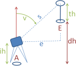
All values are always required. Missing values ih, th are padded by the default values, if any.
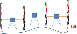
Some or all network lines may be measured twice , i.e.
In this case you simply specify two columns for height difference dh or the zenith angle v . The other quantities in the measurement record must not appear twice here. For the third case the following is assumed: The values of the instrument height ih and the target height th are only specified for AE and in the backsight EA they must be exactly interchanged. If this condition is not met, please specify means or use the method described below.
It is not necessary to change the sign of the height difference in backward direction EA. For the height difference in forward direction AE the sign of the first value is assumed. Therefore, two forward directions could have been measured. Your case is recognised by the signs of the first pair of values. (Theoretically it may happen that the height differences of the first pair are so small, that the recognition fails. In the extreme case they may be zero. Then a different record of the measurement list should be shifted to the front.)
The network lines measured twice may also be specified in two separate measurement records. This practice allows greater flexibility. In the same way you may specify network lines measured more than twice: each measurement in a separate record.
Examples: The following inputs yield identical results (right column: Angle unit = Grad):
| geometric network | trigonometric network |
|---|---|
| // from to dh1 dh2 l pdh A E 16.10 16.11 2306 1 |
// from to v1 v2 e ih th pdh A E 92.1402 92.1418 88.2306 1.54 1.66 1 |
| // from to dh1 dh2 l pdh A E 16.10 -16.11 2306 1 |
// from to v1 v2 e ih th pdh A E 92.1402 107.8582 88.2306 1.54 1.66 1 |
| // from to dh l pdh A E 16.10 2306 1 E A -16.11 2306 1 |
// from to v e ih th pdh A E 92.1402 88.2306 1.54 1.66 1 E A 107.8582 88.2306 1.66 1.54 1 |
Multiple measured network lines enter the adjustment as separate observations , which is generally recommended. If you want to let them enter as mean values, please get them yourself. In the examples above the records could read:
| geometric network | trigonometric network |
|---|---|
| // from to dh l pdh A E (16.10+16.11)/2 2306 1 |
// from to v e ih th pdh A E (92.1402+92.1418)/2 88.2306 1.54 1.66 2 |
Take care not to specify the multiple measured network lines as a constraint, otherwise there wil be a contradiction of the probably different values.
Here observations of the adjustment are the given height differences dh or the height differences computed from zenith angles v and distances e or s as well as the heights of known adjustable points. Accuracy measures are needed for all of them.
Also for trigonometric vertical networks these accuracy measures refer to the adjustable height difference dh, i.e. they include measurement errors in the instrument height and target height.
Correlated observations are not supported at the moment.
There are multiple opportunities, how to define the stochastic model via the selection of column format:
as given above or from standard deviations or all unity
For the definition of weights for height differences you can indirectly use
Then, for each network line please specify such a value. For this purpose you select the respective column format. You can specify how the weights are derived from distances or lengths of lines. Each height difference without length of line is treated as fixed, just as having standard deviation zero or weight ''INF''. Lengths of lines must not be specified in the same unit as the heights and height differences. Distances must have the same unit as heights and height differences. All values must be positive.
If you selected such an option and in addition you specify explicite standard deviations or weights then you obtain an error message.
For heights of known, movable points you specify a standard deviation in the same unit as the heights or a weight, as described above. Heights without accuracy measure or with standard deviation zero or weight ''INF'' are treated as error-free and fixed in the adjustment.
The weights of heights and height differences must agree. A variance component estimation is not yet implemented.
If zero standard deviations or weight ''INF'' is assigned to a height difference then they act as constraints. It may happen that these constraints contradict. This case arises if these height differences
These cases cause an error. Use height differences as constraints with care.
The computation is performed such that either the startpoint or the endpoint of each such line is eliminated from the list of adjustable points and is added after the adjustment using the constraint.
The adjustment is performed according to the method of least squares. Free vertical networks are adjusted with the datum constraint that the sum of all adjusted heights is equal to zero.
The documented results contain the residuals, the adjusted values, the corresponding a posteriori standard deviations and the redundancy parts.
If a priori standard deviations are given for all heights and height differences (e.g. zero), then you compute the a priori standard deviations of the adjusted values by dividing the corresponding a posteriori values by σo . You find such a case in the example Trigonometric levelling line.

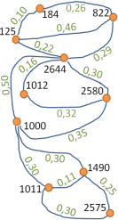
In the third semester of the curriculum Geomatics of the  parts of the campus vertical network are measured by spirit levelling.
As a result the height differences dh in metres and lengths of the lines l
in kilometres given below have been obtained.
Each levelling line has been measured multiple times, here between two and six times.
These observations should be adjusted as a free vertical network.
As a result for a single line of length 1 km (unit weight) we obtain a posteriori
standard deviation of 0.47 mm
. All partial redundancies are above 0.7
, such that the network enjoys sufficient reliability.
All residuals amount to less than 0.5 mm
. For the point heights this yields a posteriori standard deviations up to a maximum of
0.15 mm.
| from | to | Δh [m] | l [km] | from | to | Δh [m] | l [km] | from | to | Δh [m] | l [km] |
|---|---|---|---|---|---|---|---|---|---|---|---|
| 2580 | 2644 | -0.05638 | 0.37 | 1011 | 2575 | 9.70155 | 0.29 | 822 | 2644 | -2.91135 | 0.28 |
| 2580 | 2644 | -0.05592 | 0.28 | 1000 | 1011 | 8.80803 | 0.29 | 822 | 2644 | -2.91116 | 0.30 |
| 2580 | 2644 | -0.05659 | 0.37 | 1000 | 1011 | 8.80839 | 0.30 | 184 | 822 | 3.11445 | 0.25 |
| 2580 | 2644 | -0.05609 | 0.27 | 1000 | 1011 | 8.80838 | 0.33 | 184 | 822 | 3.11462 | 0.27 |
| 1490 | 2575 | 9.79288 | 0.25 | 1000 | 1011 | 8.80852 | 0.29 | 184 | 822 | 3.11540 | 0.25 |
| 1490 | 2575 | 9.79311 | 0.26 | 1000 | 1490 | 8.71692 | 0.28 | 184 | 822 | 3.11474 | 0.26 |
| 1012 | 2580 | 0.60757 | 0.32 | 1000 | 1490 | 8.71712 | 0.29 | 125 | 184 | 0.61625 | 0.11 |
| 1012 | 2580 | 0.60767 | 0.31 | 1000 | 1490 | 8.71700 | 0.28 | 125 | 184 | 0.61652 | 0.10 |
| 1012 | 2580 | 0.60785 | 0.32 | 1000 | 1490 | 8.71724 | 0.33 | 125 | 184 | 0.61656 | 0.10 |
| 1012 | 2580 | 0.60800 | 0.31 | 1000 | 2580 | -0.60227 | 0.32 | 125 | 184 | 0.61632 | 0.11 |
| 1012 | 2644 | 0.55162 | 0.16 | 1000 | 2580 | -0.60220 | 0.38 | 125 | 184 | 0.61656 | 0.10 |
| 1012 | 2644 | 0.55167 | 0.16 | 1000 | 2580 | -0.60257 | 0.29 | 125 | 184 | 0.61669 | 0.10 |
| 1012 | 2644 | 0.55163 | 0.16 | 1000 | 2580 | -0.60284 | 0.36 | 125 | 822 | 3.73164 | 0.46 |
| 1012 | 2644 | 0.55177 | 0.16 | 1000 | 2644 | -0.65811 | 0.47 | 125 | 822 | 3.73182 | 0.46 |
| 1011 | 1490 | -0.09163 | 0.10 | 1000 | 2644 | -0.65810 | 0.51 | 125 | 2644 | 0.82011 | 0.21 |
| 1011 | 1490 | -0.09118 | 0.12 | 1000 | 2644 | -0.65860 | 0.49 | 125 | 2644 | 0.82042 | 0.22 |
| 1011 | 1490 | -0.09169 | 0.10 | 822 | 2644 | -2.91118 | 0.28 | 125 | 2644 | 0.82039 | 0.28 |
| 1011 | 1490 | -0.09140 | 0.12 | 822 | 2644 | -2.91111 | 0.30 | 125 | 2644 | 0.82062 | 0.22 |
| 1011 | 2575 | 9.70153 | 0.31 |

| from | to | height difference |
slope distance | target height |
|---|---|---|---|---|
| 1 | A | 105.545 | 55.454 | 1.400 |
| 1 | 2 | 95.112 | 71.689 | 1.400 |
| 3 | 2 | 103.230 | 49.528 | 1.400 |
| 3 | 4 | 92.751 | 65.666 | 0.005 |
| 4 | 3 | 107.239 | 65.666 | 0.005 |
| 4 | 5 | 96.345 | 78.300 | 0.005 |
| 5 | 4 | 103.645 | 78.300 | 0.005 |
| 5 | E | 99.300 | 45.650 | 1.400 |
Let us consider the displayed levelling line with a leap station at point 2, i.e. no instrument has been erected at this point and consequently at point 1 no reflector was needed. At the points 3,4,5 there was in turn a station with instrument and a reflector position. Heights are given for the levelling bechmarks A by H=116.10 and E by H=123.06 . The reflector at A, 2 and E always has a target height of th=1.40 . The points 1,3,4,5 are not marked, such that we refer the heights to the tilt axis of the instrument: ih=0.00 . However, the reflection point is always 0.005 above the tilt axis, such that on the points 3,4,5 there is a target height of th=0.005 to consider. The obtained measurement values are shown at the right.
Residuals are computed for the height differences with magnitudes up to 0.0017 . The resulting height differences of the new points 1,2,3,4,5, obtain a posteriori standard deviations up to 0.0012.
The same example is also used for the
Universal computer
and may be computed. However, the results are not fully identical because
computes a robust adjustment.
The deviations in the final heights amount up to 0.0004.
| point | Vertical networks | Universal computer | ||
|---|---|---|---|---|
| name | adj. height | stddev. | height (median) | IQR |
| 1 | 122.3238 | 9.1e-4 | 122.3237 | 0.0024 |
| 2 | 126.4233 | 0.0012 | 126.4230 | 0.0024 |
| 3 | 130.3350 | 0.0012 | 130.3347 | 0.0024 |
| 4 | 137.7910 | 0.0011 | 137.7906 | 0.0025 |
| 5 | 142.2778 | 7.7e-4 | 142.2779 | 0.0024 |

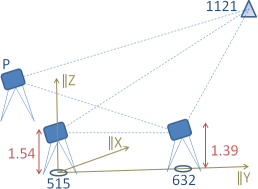
This example has been computed with the Universal computer before. We now adjust the measurements as a trigonometric network. For this purpose we use the slope distances obtained in the universal computer. The known point height of 515 and 632 are set as fixed. The planar coordinates are used only for plotting the network on the canvas.
During the computation a warning is issued that observations are found between fixed points, which are ignored. These are the two observations between the points 515 and 632 All observations are well reliable (redundancy parts ≥ 0.45). The adjusted heights of the inaccessible point 1121 is obtained as 201.1118 with a standard deviation of 0.0014.
The same example is also used for
Universal computer
and may be computed. However, the results are not fully identical because
computes a robust adjustment and determines all three spatial coordinates.
The deviations in the final heights amount up to 0.07.
Adjustment with observation equations
and can be re-adjusted with . This yields the following advantages:
Forthcoming: More tools will provide this option.
The names of the observations are A°E and the names of the parameters are the names of the adjusted points. If you use height differences as constraints then they do not show up as observations, but as constraints for parameters.
Determine the standard deviation of the adjusted height difference of the points 125 and 2575 in the Campus subnetwork of the HTW Dresden as a free spirit levelling network. Solution: 0.22 mm.
In a Vertical network the accuracy of adjusted, unmeasured height differences should be computed. You could load the vertical network to like in the preceeding trick and specify the height differences as functions of adjusted parameters (heights). It is simpler to specify the height differences directly in the height network as measurement with weight zero or standard deviation ''INF''. Then the values do not take part in the adjustment, but you obtain the adjusted values and also their accuracy.
|
|
|
|