Page contents

Accuracy measures Application of propagation laws Radius of circular arc Error propagation with the Universal computer and with Trilateration Arcs intersection In the library

≡ START First steps Deutsch

In geodesy we not only compute unknown quantities, but we also estimate, how accurate or inaccurate such quantities are obtained. Computed quantities inherit their deviations, the so-called errors, from the quantities, from which they are computed. These quantities may have been measured and are affected by measurement errors or computed from other quantities and so have again inherited their deviations. It is said that errors propagate. Both amplification as well as dilution of errors is possible.

It is important to carry out error propagations

1. to specify the accuracy of computed quantities
2. to determine the required accuracy of measured values and
3. to optimize measurement arrangements.

These three goals are attained by the application of propagation laws.

≡ START First steps Deutsch Accuracy measures

Accuracies may be expressed by numbers in different ways. IN DUBIO PRO GEO works with the following three accuracy measures:

standard deviation	Std	formerly known as mean error
maximum absolute deviation	Max	worst case error
weight	Wgt	a relative accuracy measure

In geodesy the standard deviation is more popular because the maximum absolute deviation is difficult to estimate or yields values, which are theoretically possible, but only by a chain of worst cases.

• Accuracy measures must not be negative, and weights must not be zero.
• In case of missing accuracy measures the related quantities are treated as error-free.
• Deviation measures must not be arbitrary large, otherwise you may get incorrect results and in extreme cases even no result at all, but an error message.

A simple test for deviations to be sufficiently small is to repeat the computation with all accuracy measures halved and to check that also all computed measures are approximately halved.

≡ START First steps Deutsch Application of propagation laws

For each accuracy measure there is a corresponding propagation law. Please find the theoretical basics explained here: (Sorry, only in German)

If for any uncertain start quantity a related measure of uncertainty is available then for some computation tools ( ) these measures may be specified and the related accuracy measures for all computed quantities are obtained. This requires the start quantities to be statistically uncorrelated. Practically this means that these deviations ultimately result from measurement errors, but each of them has affected only one start quantity.

≡ START First steps Deutsch Radius of circular arc

How accurate can we determine the radius of a circular arc from tape measurements of the chord segments AQ and QE and chord offset PQ? From experiences we obtain for all three measurement values a standard deviation of 0.03 The result is a radius of 12.57 with a standard deviation of 0.18.

and Compute

If we assume instead or additionally a maximum absolute deviation of the tape measurements of 0.1 each, then we obtain for the radius a maximum absolute deviation of 0.86.

and Compute

In both cases the deviations are significantly amplified. This effect is even stronger for shallow arcs, which occur practically e.g. in traffic infrastructure construction.

If we would not know for sure, which standard deviation should be assigned to the tape mesurements, but only that they have a certain ratio, then we could work with weights. If these standard deviation are all equal, we choose the weight 1 for all measurements and compute the weight propagation. As a result we obtain for the radius the relatively small weight 0.028 which indicates a bad error propagation.

and Compute

If we would try to determine the radius from measurements of the long chord AE and the two short chords AP and PE (⇑ figure) with the same accuracy, i.e., with the same weight 1, the we would obtain by weight propagation for the radius the even smaller weight 0.0034 This measurement setup is therefore even less recommendable.

and Compute

Interesting enough, all these computations can as well be performed with . The triangle AEP is computed. The arc's radius equals the radius of circumcircle of this triangle. As an example we present the first computation in this version:

and Compute

≡ START First steps Deutsch Error propagation with the Universal computer and with Trilateration

Although the does not support the error propagation directly, it is possible to skillfully compute an error propagation also here. Let us assume, we have n inaccurate start quantities (coordinates and/or measurements). You run the computation n+1 times, one time with unchanged start values and n times with one start value changed by its standard deviation or maximum absolute deviation, one after the other. The differences Δ_i of the desired results with respect to the first run of the computation are totalize according to the law of error propagation:

for standard deviations	σ²= Δ1² +…+ Δn²
for maximum absolute deviations:	Δ=|Δ1|+…+|Δn|

If you rename the points wíth changed coordinates and append them to the coordinate list and if you also assign different names to the n+1 results of the unknown points, then you can run the n+1 computations in the in a single flow .

The same works just as well with the computation tool .

≡ START First steps Deutsch Arcs intersection

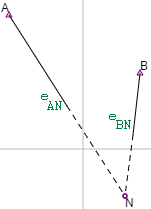
Let us consider an arcs intersection with two known points A and B and an unknown point N as well as two measured horizontal distances e_AN = 11.436; e_BN = 6.576. The four position coordinates have standard deviations of 0.03 and both distances have standard deviations of 0.01. Consequently, we have 6 inaccurate start quantities X_A,Y_A, X_B,Y_B,e_AN,e_BN. Thus, the list of known points may read:

      Y     X
A   16.10 17.11 // unchanged point
B   23.06 14.02 // unchanged point
AY  16.13 17.11 // Y-changed point A
BY  23.09 14.02 // Y-changed point B
AX  16.10 17.14 // X-changed point A
BX  23.06 14.05 // X-changed point B

Now we compute the 7 arcs intersections in a single workflow by the and to the 7 results for the unknown point we assign the pointnames N,N1,N2,…,N6 . Every arcs intersection has two solutions. They combine to a total of 2⁷=128 solutions. But it is sufficient to consider only the first one. All other solutions yield the same accuracies.

and Compute with

and Compute with

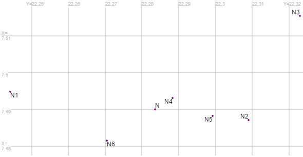
It is easy to display the spatial distribution of the 7 computed points by storing them in a coordinate list and looking at the canvas. The largest impact is made by the X coordinates of the known points A (→N1), B (→N3):

Now we must compute the differences Δ_i . This can be supported by and computation of a translation, such that N is moved to the origin of the coordinate system. The transformed coordinates of the other 6 points are immediately the desired differences. Finally, we obtain for the unknown point N by application of the law of error propagation for standard deviations:

σ_Y=(0.039²+0.025²+0.039²+0.005²+0.016²+0.013²)^½=0.065
σ_X=(0.005²+0.003²+0.025²+0.003²+0.002²+0.008²)^½=0.028

If the given deviations would have been maximum absolute deviations then by application of the law of related error propagation we would obtain:

Δ_Y=0.138; Δ_X=0.047

In both cases the deviations amplify mainly in the Y coordinate.

Did you know? Place mousepointer over terms marked with to get their meaning.

≡ START First steps Deutsch